


Ever wondered what stats mean and when the right time was to use them was?
Well, this is the podcast/video for you!
In this bonus episode, I am joined by Clive Palmer to talk about advanced stats, and how they help us to understand the game. Learn how the stats work, what the limitations are, and what context is needed for the stats.
Below is the very detailed notes and explanations I wrote to prepare for this podcast.
At the very bottom for premium subscribers is the video recording that we made as well. (if you subscribe to the Arsenal Vision Podcast Patreon this should also be available to you on that channel)
Expected Goals (xG):
This is probably the advanced stat one that people are most familiar with but it is probably still a bit understood.
I think the resistance to the idea behind rating chances has broken down. We all naturally have an intuitive sense of when a chance is high or low-quality. For example the Gabriel Jesus goal against Manchester United. We KNOW this is a clear chance and that there is a high probability of scoring here.
But what is the estimate of scoring here?
For this shot in my expected goals model, it is rated as 67% chance of being converted, which is going to be on the higher side for what chances will end up being rated.
The largest factors for a shot’s rating is the distance from goal, the angle of the goal for the player to aim at, and if it was taken with feet, head or other.
The information for this comes from event data that gives the time and location of every on-ball action on the field. From this, we can infer information about the chance and use that to compare it to how those factors of applied to shots with similar characteristics.
This shot is from a fast break situation, which helps tell that the defense is not going to be set and it a more dangerous situation. The speed of this move is 7.3 yards per second making this a very direct attack with is another positive indicator that the defense has been unsuccessful in slowing the attack down.
Jesus completes a dribble before he shoots this is a major positive for his chance as it is a clear indicator that he has opened up space for a shot.
This is also given the “big chance” indicator by Opta and that is a bit of a cheat that helps that this is not pressured and a one-on-one.
One of the major limits of doing this with the regular event data is that the model is blind to where the other players are and information needs to be inferred from other characteristics.
We see this when he takes the shot:
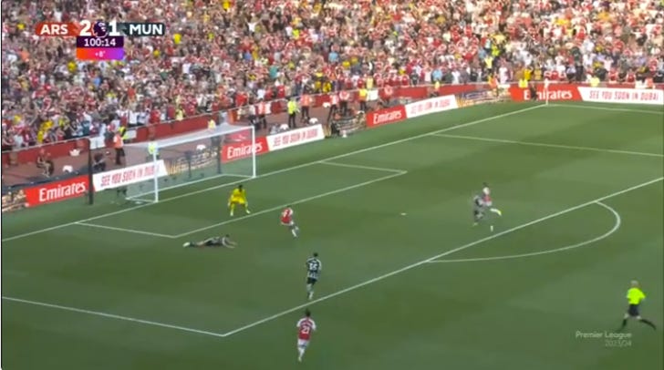
The model from the event data only knows this and has to guess as to everything else from the proceeding events and the characteristics of the shot:

This is an obvious shortcoming and why when you see the xG for a shot, especially from ones that don’t have tracking elements (for example Statsbomb uses freeze frames to also show where all the players are in the frame for the events that they capture. The newer Opta data also uses something similar to get around this) it should come with pretty large error bars for the estimate of the “true” probability for the shot. With this shot we can make some decent assumptions, it’s a direct/fast break so minimal defenders back. Jesus made a dribble before he shot which probably means he isn’t under pressure when he shoots but it is still a bit of guesswork on to just how open it might be.
When to Use xG
You will see xG used in a number of different places and ways. One of the more popular is after a match; I post a couple of different illustrations of the xG for a match that I think are helpful for describing the game.

The first is the xG shot map, which plots all of the shots and goals for each team and the size of the dot corresponds to the xG value. This gives a nice picture of where the shots took place and how dangerous those shots were. There are a number of different ways that a team can accumulate the different xG values and seeing the shots helps provide more information and context for the number.
The next popular type is the xG race chart.

This shows the timing and value of the different shots that each team took. It can help illustrate a number of different things that might not be obvious from a shot chart alone. First is that game state (the score, and number of players on the field) matters and will change the strategy for teams. Second, it also helps describe and get a feel for how the game has gone from the total chance creation.
With my running xG charts I also add in error bars, which is the shaded area to help illustrate the uncertainty that comes with each shot that we identified earlier.
Single match xG is still better thought of as a descriptive tool, it tells you what happened in a match. It can help tell you if a team was better or if perhaps a win was lucky but that is just part of the picture (we will have more stats on this kind of thing later). A single match can be pretty random with lots of small things affecting if a clear-cut chance happens or not. Over more matches, the signal becomes stronger and the value of xG starts to shine through.
Using xG in the season
One of the things that xG is good at, is that it is a better predictor of future goals scored/allowed for a team than other measures, especially in smaller sample sizes. When you get into the 8-12 match range the advantage for xG is at its highest over goals in predictive power, with goals closing the to be nearly as good as xG as the season progresses further.
This is especially helpful when there is a big deviation from expected and actual production during the period in question, as the better bet is that future production will be closer to xG than goals.
Even better however is using a combination of the two with weights of 70/30 because goals also have important information about a team. This is why you will see me use charts like this in the season.

Goals provide information, they are the main component of what a team is trying to do in a game towards winning points
One other thing is that aggregation can hide information with outlier games having an outsized effect on things. For situations like this I have another chart that I think is a helpful wau to look at a team.

This chart plots a team’s xG for and against over the course of the season. For Arsenal last season they were consistently better than their opponents with just a handful of times where they were outplayed and one really big outlier performance.
This is another one that you can also use the weighted xG and Goals as well to help get the story of the season for the team.

Post Shot Expected Goals/Goalkeeping Metrics
Post-Shot xG (PSxG) or xG On Target (xGOT) are models that look to measure the xG value of a shot but instead of stopping at the moment that shot is taken it also looks at where the shot is in relation to the frame of the goal.
For a post-shot xG model, the biggest factors are still the distance and angle of the shot, but also now also the z and y coordinates of where it is estimated to cross the goal line.
PSxG models do not take into account the positioning of the keeper (by design because better positioning is a skill that will help a keeper save more than expected) and some have information about how hard the bull has been struck but that is not available in the more simple event data.

When to Use PSxG
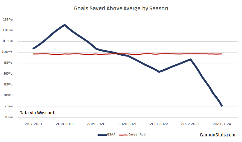
Post-shot xG is also a noisy stat where finding the signal of how good a goalkeeper is at keeping out shots or a player is at placing their shots is harder to estimate. Season to season a goalkeeper’s goals prevented compared to expected (PSxG- Actual Goal) is in the +/- 0.2 goals prevented per 90 range, that is a BIG variation from season to season.
If for example, you have Aaron Ramsdale who for his career is roughly at 99% for goals saved compared to average, in a single season it wouldn’t be out of the ordinary to see that fluctuate to between 115% and 75% and that is what he has done for his career!
I have not seen the same level of estimates of when exactly these type of stats become more reliable with confidence intervals that are not huge yet like what has been done with finishing where you can start seeing a signal at the 75+ shots range but realistically a few hundred shots to have confidence about a player’s finishing skill.
My intuition is that it is probably in the 150+ to start seeing a signal and in the 300 or more range to get a more reliable idea but I have not had the time to put this to the test. A project for another day.
So given the above information, it does feel like goalkeeper stats are ones that should come with pretty high error bars around them, especially for a single shot, a single match, or even a season.
They can be thought of I think as at best rough estimates but beyond that my confidence with them comes with large caveats.
Expected Threat (xT)/Goal Probability Added(GPA)
This was a popular question when I asked what people wanted to learn about.
Expected Threat was created by Karun Singh (now employed by Arsenal) and has become one of the more popular ways of calculating on-ball actions. If you are interested in the nitty-gritty of how it works he has a nice write-up on the methodology on his blog.
The shorter explanation is that the pitch is laid out into zones and a player is credited with the difference in value between those zones as it is moved through passing and carrying.
I have been doing something similar for a while and my first stab at something like this going back to my 2017 Passing Progression Value Added and have evolved my work into what I call Goal Probability Added.
My model also works off of zones and the value of each is trained from the xG created in a possession after the ball has been in that zone, along with the probability that the other team will create xG from you having possession in that zone. Giving you a pitch that looks something like this:

Most of the field is not very valuable, with pretty minor increases until you get within 25 or so yards of goal. You will also see that possession in your own box is negative meaning the other team is more likely to score when the ball is there than you are.
My model also takes into account the failure of an action and how that changes both teams’ chances of scoring.

I took a lot of inspiration from the work done on by American Soccer Analysis and their Goals Added model for direction on certain questions. My model also breaks things down into similar parts, passing, receiving, carrying, dribbling, and shooting.

I have started breaking down defensive actions as well for how that changes the opposing team’s actions but don’t publish that regularly with match reports.
With this you can create fun sequence-type charts that show the change in goal probability as the ball moves around the pitch. This is the first goal in Arsenal’s 3-1 win against Manchester United scored by Martin Odegaard.

Most of the buildup play is low value because it is still far away from goal. The play starts to become more valuable as it gets into the final third. From there the pass into Eddie Nketiah in the half-space adds 3% to the chance of scoring, his pass into the box to Gabriel Martinelli adds 8% and then his cross adds 20% with the very good finish adding another 5%.


